Looping through and fitting multiple impedance data sets

import glob
import numpy as np
import os

1. Find all files that match a specified pattern

Using a search string to find .z files that contain “Circuit” at the beginning and EIS towards the end

directory = r'../../../data/'
all_files = glob.glob(os.path.join(directory, 'Circuit*EIS*.z'))
all_files

['../../../data/Circuit3_EIS_1.z',
 '../../../data/Circuit1_EIS_2.z',
 '../../../data/Circuit2_EIS_1.z',
 '../../../data/Circuit3_EIS_2.z',
 '../../../data/Circuit1_EIS_1.z',
 '../../../data/Circuit2_EIS_2.z']

2. Use preprocessing module to read in ZPlot data

from impedance import preprocessing
# Initialize some empty lists for the frequencies and Z data
freqs = []
Zs = []

# Now loop through file names in our list and extract data one by one
for filename in all_files:
    f, Z = preprocessing.readZPlot(filename)
    freqs.append(f)
    Zs.append(Z)

# Check to see if we extracted data for all the files
print(np.shape(Zs), np.shape(all_files))

(6,) (6,)

3. Create a list of circuit models

from impedance.models.circuits import CustomCircuit
# This data comes from dummy circuits I made to check measurement bias in
# our potentiostat, so I know a priori its an R-RC circuit

circuits = []

circ_string = 'R0-p(R1,C1)'
initial_guess = [100, 400, 1e-5]

# Now loop through data list to create circuits and fit them
for f, Z, filename in zip(freqs, Zs, all_files):
    name = filename.split('/')[-1]
    circuit = CustomCircuit(circ_string, initial_guess=initial_guess, name=name)
    circuit.fit(f, Z)
    circuits.append(circuit)

We now have a list of our circuit class objects, all fit to different sets of data. As you may notice from the file names, there are three unique circuits each with a replicate set of data. We expect each of the replicates to fit similarly.

for circuit in circuits:
    print(circuit)

Name: Circuit3_EIS_1.z
Circuit string: R0-p(R1,C1)
Fit: True

Initial guesses:
     R0 = 1.00e+02 [Ohm]
     R1 = 4.00e+02 [Ohm]
     C1 = 1.00e-05 [F]

Fit parameters:
     R0 = 1.51e+03  (+/- 2.62e+00) [Ohm]
     R1 = 4.63e+03  (+/- 3.14e+00) [Ohm]
     C1 = 2.02e-08  (+/- 5.39e-11) [F]


Name: Circuit1_EIS_2.z
Circuit string: R0-p(R1,C1)
Fit: True

Initial guesses:
     R0 = 1.00e+02 [Ohm]
     R1 = 4.00e+02 [Ohm]
     C1 = 1.00e-05 [F]

Fit parameters:
     R0 = 2.91e+01  (+/- 3.58e-02) [Ohm]
     R1 = 4.67e+01  (+/- 4.64e-02) [Ohm]
     C1 = 1.04e-05  (+/- 2.91e-08) [F]


Name: Circuit2_EIS_1.z
Circuit string: R0-p(R1,C1)
Fit: True

Initial guesses:
     R0 = 1.00e+02 [Ohm]
     R1 = 4.00e+02 [Ohm]
     C1 = 1.00e-05 [F]

Fit parameters:
     R0 = 1.50e+02  (+/- 3.23e-01) [Ohm]
     R1 = 5.02e+02  (+/- 3.57e-01) [Ohm]
     C1 = 3.12e-08  (+/- 7.79e-11) [F]


Name: Circuit3_EIS_2.z
Circuit string: R0-p(R1,C1)
Fit: True

Initial guesses:
     R0 = 1.00e+02 [Ohm]
     R1 = 4.00e+02 [Ohm]
     C1 = 1.00e-05 [F]

Fit parameters:
     R0 = 1.51e+03  (+/- 2.68e+00) [Ohm]
     R1 = 4.63e+03  (+/- 3.21e+00) [Ohm]
     C1 = 2.02e-08  (+/- 5.52e-11) [F]


Name: Circuit1_EIS_1.z
Circuit string: R0-p(R1,C1)
Fit: True

Initial guesses:
     R0 = 1.00e+02 [Ohm]
     R1 = 4.00e+02 [Ohm]
     C1 = 1.00e-05 [F]

Fit parameters:
     R0 = 2.91e+01  (+/- 3.63e-02) [Ohm]
     R1 = 4.67e+01  (+/- 4.69e-02) [Ohm]
     C1 = 1.04e-05  (+/- 2.95e-08) [F]


Name: Circuit2_EIS_2.z
Circuit string: R0-p(R1,C1)
Fit: True

Initial guesses:
     R0 = 1.00e+02 [Ohm]
     R1 = 4.00e+02 [Ohm]
     C1 = 1.00e-05 [F]

Fit parameters:
     R0 = 1.50e+02  (+/- 3.19e-01) [Ohm]
     R1 = 5.02e+02  (+/- 3.53e-01) [Ohm]
     C1 = 3.12e-08  (+/- 7.70e-11) [F]

Now we’ll get the impedance predicted by the fit parameters

fits = []
for f, circuit in zip(freqs, circuits):
    fits.append(circuit.predict(f))

4. Plot the data and fits

Now we can visualize the data and fits. For now we’ll place them all on the same axis

import matplotlib.pyplot as plt
from impedance.visualization import plot_nyquist, plot_bode

fig, ax = plt.subplots()

for fit, Z in zip(fits, Zs):
    # Plotting data
    plot_nyquist(ax, Z)

    # Plotting fit
    plot_nyquist(ax, fit)

plt.show()

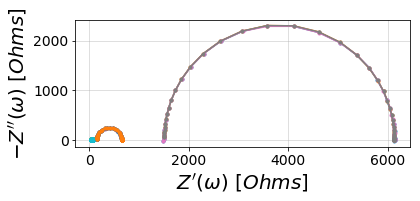
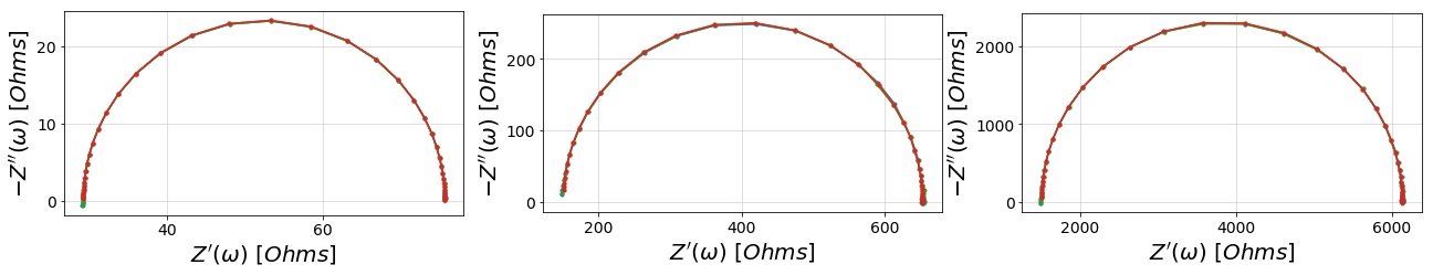
Since the circuits have different orders of magnitude impedance, this looks bad so let’s put each pair of data on separate axes.

# Nyquist plots
fig, axes = plt.subplots(ncols=3, figsize=(22,6))
for circuit, Z, fit in zip(circuits, Zs, fits):
    n = int(circuit.name.split('Circuit')[-1].split('_')[0])
    plot_nyquist(axes[n - 1], Z)
    plot_nyquist(axes[n - 1], fit)

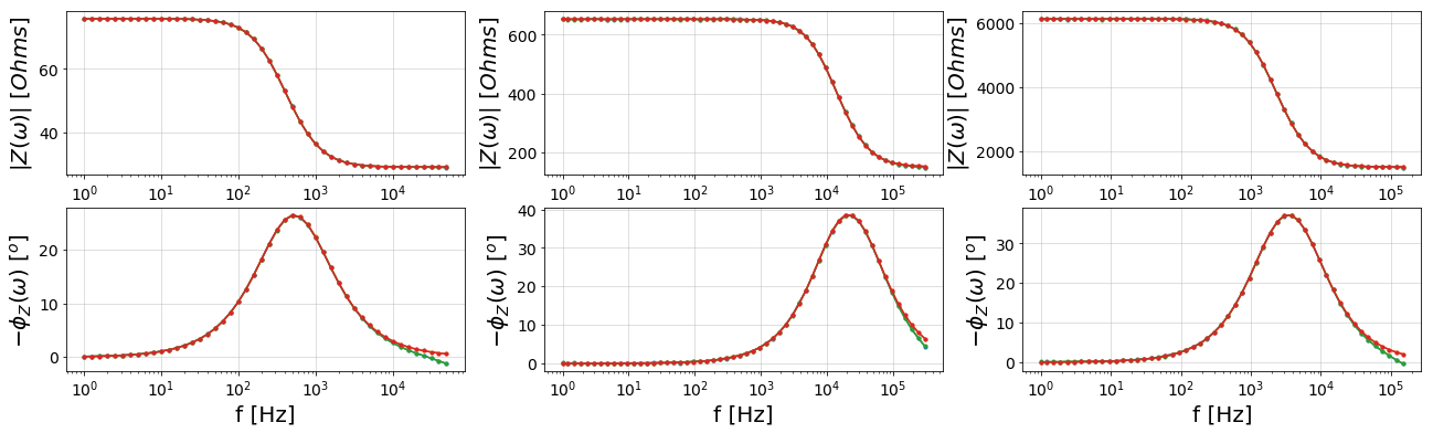
# Bode plots
fig, axes = plt.subplots(nrows=2, ncols=3, figsize=(22,6))
for circuit, f, Z, fit in zip(circuits, freqs, Zs, fits):
    n = int(circuit.name.split('Circuit')[-1].split('_')[0])
    plot_bode([axes[0][n - 1], axes[1][n - 1]], f, Z)
    plot_bode([axes[0][n - 1], axes[1][n - 1]], f, fit)

plt.show()