Getting started with `impedance.py`¶

impedance.py is a Python package for analyzing electrochemical impedance spectroscopy (EIS) data. The following steps will show you how to get started analyzing your own data using impedance.py in a Jupyter notebook.

Hint

If you get stuck or believe you have found a bug, please feel free to open an issue on GitHub.

Step 1: Installation¶

If you already are familiar with managing Python packages, feel free to skip straight to Installing packages. Otherwise, what follows is a quick introduction to the Python package ecosystem:

Installing Miniconda¶

One of the easiest ways to get started with Python is using Miniconda. Installation instructions for your OS can be found at https://conda.io/miniconda.html.

After you have installed conda, you can run the following commands in your Terminal/command prompt/Git BASH to update and test your installation:

Update conda’s listing of packages for your system: conda update conda
Test your installation: conda list

For a successful installation, a list of installed packages appears.

Test that Python 3 is your default Python: python -V

You should see something like Python 3.x.x :: Anaconda, Inc.

You can interact with Python at this point, by simply typing python.

Setting up a conda environment¶

(Optional) It is recommended that you use virtual environments to keep track of the packages you’ve installed for a particular project. Much more info on how conda makes this straightforward is given here.

We will start by creating an environment called impedance-analysis which contains all the Python base distribution:

conda create -n impedance-analysis python=3

After conda creates this environment, we need to activate it before we can install anything into it by using:

conda activate impedance-analysis

We’ve now activated our conda environment and are ready to install impedance.py!

Installing packages¶

The easiest way to install impedance.py and it’s dependencies (scipy, numpy, and matplotlib) is from PyPI using pip:

pip install impedance

For this example we will also need Jupyter Lab which we can install with:

conda install jupyter jupyterlab

We’ve now got everything in place to start analyzing our EIS data!

Note

The next time you want to use this same environment, all you have to do is open your terminal and type conda activate impedance-analysis.

Open Jupyter Lab¶

(Optional) Create a directory in your documents folder for this example:

mkdir ~/Documents/impedance-example

cd ~/Documents/impedance-example

Next, we will launch an instance of Jupyter Lab:

jupyter lab

which should open a new tab in your browser. A tutorial on Jupyter Lab from the Electrochemical Society HackWeek can be found here.

Tip

The code below can be found in the getting-started.ipynb notebook

Step 2: Import your data¶

This example will assume the following dataset is located in your current working directory (feel free to replace it with your data): exampleData.csv

For this dataset which simply contains impedance data in three columns (frequency, Z_real, Z_imag), importing the data looks something like:

from impedance import preprocessing

# Load data from the example EIS data
frequencies, Z = preprocessing.readCSV('./exampleData.csv')

# keep only the impedance data in the first quandrant
frequencies, Z = preprocessing.ignoreBelowX(frequencies, Z)

Tip

Functions for reading in files from a variety of vendors (ZPlot, Gamry, Parstat, Autolab, …) can be found in the preprocessing module!

Step 3: Define your impedance model¶

Next we want to define our impedance model. In order to enable a wide variety of researchers to use the tool, impedance.py allows you to define a custom circuit with any combination of circuit elements.

The circuit is defined as a string (i.e. using '' in Python), where elements in series are separated by a dash (-), and elements in parallel are wrapped in a p( , ). Each element is defined by the function (in circuit-elements.py) followed by a single digit identifier.

For example, the circuit below:

would be defined as R0-p(R1,C1)-p(R2-Wo1,C2).

Each circuit, we want to fit also needs to have an initial guess for each of the parameters. These inital guesses are passed in as a list in order the parameters are defined in the circuit string. For example, a good guess for this battery data is initial_guess = [.01, .01, 100, .01, .05, 100, 1].

We create the circuit by importing the CustomCircuit object and passing it our circuit string and initial guesses.

from impedance.models.circuits import CustomCircuit

circuit = 'R0-p(R1,C1)-p(R2-Wo1,C2)'
initial_guess = [.01, .01, 100, .01, .05, 100, 1]

circuit = CustomCircuit(circuit, initial_guess=initial_guess)

Step 4: Fit the impedance model to data¶

Once we’ve defined our circuit, fitting it to impedance data is as easy as calling the .fit() method and passing it our experimental data!

circuit.fit(frequencies, Z)

We can access the fit parameters with circuit.parameters_ or by printing the circuit object itself, print(circuit).

Step 5: Analyze/Visualize the results¶

For this dataset, the resulting fit parameters are

Parameter	Value
\(R_0\)	1.65e-02
\(R_1\)	8.68e-03
\(C_1\)	3.32e+00
\(R_2\)	5.39e-03
\(Wo_{1,0}\)	6.31e-02
\(Wo_{1,1}\)	2.33e+02
\(C_2\)	2.20e-01

We can get the resulting fit impedance by passing a list of frequencies to the .predict() method.

Z_fit = circuit.predict(frequencies)

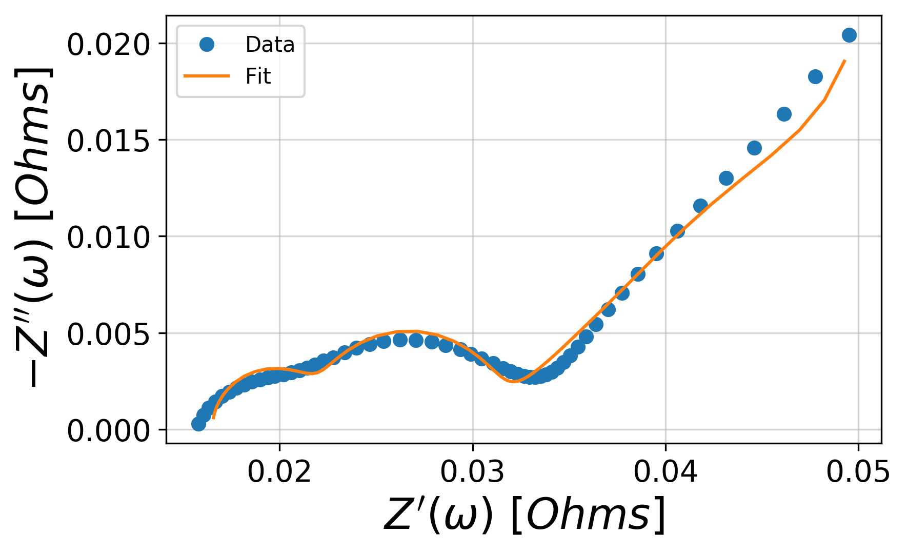
To easily visualize the fit, the plot_nyquist() function can be handy.

import matplotlib.pyplot as plt
from impedance.visualization import plot_nyquist

fig, ax = plt.subplots()
plot_nyquist(Z, fmt='o', scale=10, ax=ax)
plot_nyquist(Z_fit, fmt='-', scale=10, ax=ax)

plt.legend(['Data', 'Fit'])
plt.show()

Important

🎉 Congratulations! You’re now up and running with impedance.py 🎉

Getting started with impedance.py¶